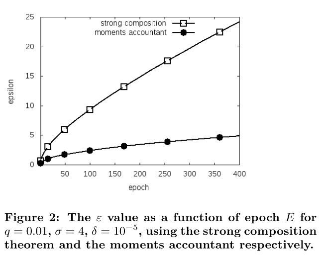
Reproducing Figure 2 from the DP-SGD paper (Abadi et al., 2016)

Dear TensorFlow Privacy Authors,

Overview

When I attempt to reproduce Figure 2 from [0], I noticed that there is a minor discrepancy between the figure itself and the numbers in the paragraph. (My code will be at the end of this post.)

I am able to reproduce the numbers in the paragraph (they are repeated two times, so I guess it’s less likely it’s a typo), i.e.,

E = 100, epsilon = 1.26 E = 400, epsilon = 2.55

However, looking at the Figure itself (also shown below for convenience), it seems that the value of epsilon at E=400 is closer to 5 than to 2.5. Am I missing something, or is this just a minor scaling issue I shouldn’t worry about?

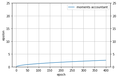
This is the plot I am getting with my code, which has the same shape as Figure 2 but different values. The epsilon values I get in my curve match the ones in the text, though.

Thank you! Andrei

Code to generate my plot (Python 3)

import math

from tensorflow_privacy.privacy.analysis.rdp_accountant import get_privacy_spent, compute_rdp
import matplotlib.pyplot as plt
import numpy as np

batch_size = 256
dataset_size = 60000    # MNIST train split

# This is the fixed value used in Figure 2.
every_q = 0.01
# every_q = batch_size / dataset_size
batch_size = dataset_size * every_q

print(f"Computed batch size for our fixed q = {every_q:.4f} is {batch_size}")

noise_stdev = 4
l2_bound = 1.0
delta = 1e-5

eps_list= []
epoch_range = np.arange(1, 401)

for epoch in epoch_range: 
    # The Renyi Divergence-based DP is computed over a bunch of orders,
    # whereby the order is the exponent in the definition.
    max_order = 64
    orders = [1 + x / 10.0 for x in range(1, 100)] + list(range(12, max_order + 1))
    rdp = np.zeros_like(orders, dtype=float)
    
    # Since our l2-bound is 1.0, this typically remains unchanged as 
    # noise_stdev.
    effective_z = sum([
        ((noise_stdev / l2_bound) ** -2) ** -0.5
    ])
    
    # Every step assumed to use the same noise magnitude and same sampling
    # probability, meaning we can avoid a costly loop and call 'compute_rdp'
    # just once, then multiply by the number of steps.
    #
    # Pretend we just worked hard and did this many steps...
    steps = epoch * dataset_size // batch_size
    # ...and then scale our RDP estimate accordingly.
    rdp = steps * compute_rdp(every_q, effective_z, 1, orders)
    
    eps, _, opt_order = get_privacy_spent(orders, rdp, target_delta=delta)
    eps_list.append(eps)
    
for E in [100, 400]:
    print("E = {}, eps = {:.2f}".format(E, eps_list[E - 1]))

plt.plot(epoch_range, eps_list, label="moments accountant")
plt.ylim((0, 25))
plt.xlabel("epoch")
plt.ylabel("epsilon")
plt.legend()
plt.grid()

# plt.gca().yaxis.tick_right()
ax2 = plt.gca().twinx()
ax2.set_ylim((0, 25))

References:

[0]: Abadi, M., McMahan, H. B., Chu, A., Mironov, I., Zhang, L., Goodfellow, I., & Talwar, K. (2016). Deep learning with differential privacy. Proceedings of the ACM Conference on Computer and Communications Security, 24-28-Octo(Ccs), 308–318. https://doi.org/10.1145/2976749.2978318

[ilyamironov]

The moments accountant and the RDP accountant are basically equivalent and must lead to identical outcomes when translated to the (eps, delta)-DP language.

I don’t have a good explanation why the figure disagrees with the text (with the text being accurate). I tested a few hypotheses, none of which checked out. Let’s chalk up the discrepancy to some buggy code that produced the graph.

Thank you for your careful reading of the paper!

[ilyamironov]

Yeah, I think it can be explained with switching the original implementation to the Renyi DP accountant.