Question on the Mode Overlap function

Hello,

I am a student researcher trying to use your software to design dielectric waveguides. I was hoping someone could please share some insight on the mode overlap function, as I think I may be using it incorrectly. I understand the mode overlap to be the coupling efficiency.

Specifically, I had a concern when simulating a straight waveguide. It is clear that the mode propagates across the waveguide, but the dB10 value of the mode overlap is about -50dB. This value practically stays the same, even as I move the probe (output port) closer to the source. I am using the functions defined in the example notebooks, (e.g., 02_Invdes_intro.ipynb).

The design:

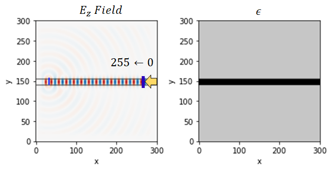
The efficiency as I move the probe closer to the source:

The mode overlap function:

def mode_overlap(E1, E2):
    """Defines an overlap integral between the simulated field and desired field
    """
    return npa.abs(npa.sum(npa.conj(E1)*E2))

What is wrong?

Thanks, Ricardo Sendrea

[momchilmm]

Yeah this is the best way to do it. You can see from the field plot that the source is not perfectly injected into the waveguide. By normalizing using the amplitude of the waveguide mode right after the source, you’re now really looking at what you want: the power transmission of that mode between the two measurement points.

[RicardoSendrea07]

The goal of the study is to observe the change of transmission (power) of a design in a frequency sweep, using the same source (fundamental mode source). I see now, that as I insert a source to the design, a mode is calculated at each iteration, i.e., the excited mode changes, as shown in my previous post.

To set this up properly, I look to use the FDTD tool offered by Ceviche. In this scenario, I can define a Gaussian source based on the same calculated eigenmode from the desired frequency and then look at the spectral power. My problem is how would I do this correctly using Ceviche?

I went ahead and put together a solution based on various examples from your packages, including using the Angler libraries. Could someone point me in the right direction, and share if I am setting this up properly?

Thanks! I appreciate your help!

# -*- coding: utf-8 -*-
"""
In this script, we implement a combination of angler and ceviche to solve a dielectric waveguide design

Following the example of the Forward Mode Grating Coupler

The script should be set in the following manner:
    1) Setup the design (here we can define input and output slice as we have had in the past)
    2) Setup a Simulation Class Object from Angler to obtain the correct sources and probes to solve the FDTD
    3) Transform the problem to FDTD and calculate the coupling efficiency
"""

# Commented out IPython magic to ensure Python compatibility.
import numpy as np
import ceviche
from ceviche import fdfd_ez, fdtd
from ceviche.modes import insert_mode
from ceviche.utils import imarr, aniplot, my_fft
import collections
import matplotlib.pylab as plt
import autograd.numpy as npa
import copy

import sys
sys.path.append('../')

from angler import Simulation, Optimization
from angler.structures import three_port, two_port
from angler.plot import *

# %load_ext autoreload
# %autoreload 2
# %matplotlib inline

""" Plotting Option """
plot_all=1
if plot_all:
    print('plotting everything...')

""" Setup the Design (as before) """    
centerFreq = 200e12
C = 3e8 #Speed of light
lam = C / centerFreq # Lambda (without considering eps)
omega=2*np.pi*centerFreq # Angular frequency of the source in 1/s
omega0 = omega
dl = (1/30)*lam # Spatial resolution in meters
#dl = 0.02 #Spatial resolition in terms of length
#Nx_l = 10
Nx_l = 10*lam
Nx=int(Nx_l/dl)+1 # Number of pixels in x-direction 
Ny=int(Nx_l/dl)+1 # Number of pixels in y-direction
Npml=int(lam/dl)+1 # Number of pixels in the PMLs in each direction
epsr_min=1.0 # Minimum value of the relative permittivity
epsr_max=3.0 # Maximum value of the relative permittivity
space= int(0.25*lam / dl) #Space between the PMLs and the design region (in pixels)
wg_width_l = lam / 2 #6 mm
#wg_width_l = 0.3 #6 mm
wg_width=int(wg_width_l / dl)+1 # Width of the waveguide (in pixels)
space_slice = 32
Slice = collections.namedtuple('Slice', 'x y')

""" Define Parameters """
#Time step setup: 
simPeriod = 1 / centerFreq              #center frequency period
total_time = 3*simPeriod              # total simulation time (s)
band = 0.01e12                          #bandwidth of signal
sigma = 1/band
t0 = 0                                  # delay (s) of pulse center from t=0

#Setup the straight waveguide
#runSteps = 201 #For frequency sweep
#freqSweep = np.linspace(1, 400, runSteps)*1e12 
centerPosition = int(Ny / 2)
epsr = epsr_min*np.ones((Nx, Ny))
epsr[:, centerPosition-int(wg_width/2):centerPosition+int(wg_width/2)] = epsr_max

#Add gap
#gap_width = 40
#epsr[centerPosition-int(gap_width/2):centerPosition+int(gap_width/2), :] = 1

#Define additional angler params
lambda0 = C / centerFreq             # free space wavelength (m)
NPML = [Npml, Npml]
pol = 'Ez'                 # polarization (either 'Hz' or 'Ez')
source_amp = 1              # amplitude of modal source (A/L0^2?)

#Setup slices
input_slice  = Slice(x=np.array(Npml+1), y=np.arange(int(Ny/2-wg_width/2-space_slice), int(Ny/2+wg_width/2+space_slice)))
output_slice = Slice(x=np.array(Nx-Npml-1), y=np.arange(int(Ny/2-wg_width/2-space_slice), int(Ny/2+wg_width/2+space_slice)))


""" Setup  Model Source / Probe """
#Setup the Angler Simulation Object
simulation = Simulation(omega, epsr, dl, NPML, pol, L0= 1)
# compute the grid size the total grid size
print("Computed a domain with {} grids in x and {} grids in y".format(Nx,Ny))
print("The simulation has {} grids per free space wavelength".format(int(lambda0/dl/simulation.L0)))
simulation.plt_eps()
plt.show()

# set the modal source and probes
simulation = Simulation(omega, epsr, dl, NPML, pol, L0= 1)
simulation.add_mode(np.sqrt(epsr_max), 'x', [int(Npml+1), int(Ny/2)], int(Ny/3), scale=source_amp)
simulation.setup_modes()

out = Simulation(omega, epsr, dl, NPML, pol, L0= 1)
out.add_mode(np.sqrt(epsr_max), 'x', [int(Nx-Npml-1), int(Ny/2)], int(Ny/3))
out.setup_modes()
J_out = np.abs(out.src)

#View fdfd simulation
(_, _, Ez) = simulation.solve_fields()
simulation.plt_abs(outline=True, cbar=True);

# get the wg mode profile as an array - change all  wg_mode to source (variable created from this line!)
source = np.flipud(np.abs(simulation.src.copy())).reshape((Nx, Ny, 1))

# compute the power in the waveguide mode for normalization
source_p = np.sum(np.square(np.abs(source)))
print('input power of {} in W/L0'.format(simulation.W_in))

# plot the wavegiude mode source array
if plot_all:
    plt.imshow(np.real(imarr(source)), cmap='magma')
    plt.title('modal source array')
    plt.xlabel('x'); plt.ylabel('y')
    plt.show()
    
""" Define the time domain simulation """

# reshape things for the FDTD
eps_base = epsr
eps_total = eps_base
eps_total = eps_total.reshape((Nx, Ny, 1))
source = source.reshape((Nx, Ny, 1))

# make an FDTD and get its time step
F_t = fdtd(eps_total, dl, [Npml, Npml, 0])
dt = F_t.dt
steps = int(total_time / dt)
times = np.arange(steps)
print('-> total of {} time steps'.format(steps))

# make a gaussian source: following Ceviche
gaussian = lambda t: np.exp(-(t - t0 / dt)**2 / 2 / (sigma / dt)**2) * np.cos(omega * t * dt)
source_fn = lambda t: np.abs(source) * gaussian(t)
spect_in = np.square(np.abs(my_fft(gaussian(times))))
delta_f = 1 / steps / dt
freq_x = np.arange(steps) * delta_f

# compute normalization power spectrum
F_norm = fdtd(eps_base.reshape((Nx, Ny, 1)), dl, [Npml, Npml, 0])
measured = []
print('-> measuring spectral power in for base waveguide')
for t_index in range(steps):
    if t_index % 1000 == 0:
        print('   - done with time step {} of {} ({}%)'.format(t_index, steps, int(t_index / steps * 100)))
    fields = F_norm.forward(Jz=source_fn(t_index))
    measured.append(npa.sum(fields['Ez'] * np.flipud(source)))

# get spectral power
print('-> computing FFT')
measured_f = my_fft(npa.array(measured))
spect_in_measure = npa.square(npa.abs(measured_f)) / source_p   # this is to normalize by the straight waveguide mode power

# plot the source amplitude in the time domain
if plot_all:
    plt.plot(times * F_t.dt / 1e-15, gaussian(times))
    plt.title('source')
    plt.xlabel('time (femtoseconds)')
    plt.ylabel('amplitude')
    plt.show()

# plot the source power in the frequency domain
if plot_all:
    plt.plot(freq_x / 1e12, spect_in, label='direct from source')
    plt.plot(freq_x / 1e12, spect_in_measure, label='measured')
    plt.xlabel('frequency (THz)')
    plt.ylabel('power')
    plt.xlim((1, 400))
    #plt.xlim((180, 210))
    plt.legend()
    plt.show()

if plot_all:
    if False: # takes an FDTD simulation to generate.
              # Make true if you want to see `num_panels` field plots at even intervals
        aniplot(F_t, source_fn, steps, component='Ez', num_panels=5)


""" SPECTRAL POWER COMPUTATION """

# reshape other things for FDTD
eps_base = eps_base.reshape((Nx, Ny, 1))

def spectral_power(ff):
    """ This function computes the spectral power as a function of fill factor
        will autograd/differentiate this with FMD (cevijacobian function)
    """

    # setup FDTD using explicit projection into permittivity
    eps_total =  eps_base
    F = fdtd(eps_total, dl, [Npml, Npml, 0])

    # compute fields at each time step at the source above
    # note: we're solving the reciprocal problem of a waveguide -> free space coupler
    measured = []
    print('-> running FDTD within objective function')
    for t_index in range(steps):
        if t_index % 1000 == 0:
            print('   - done with time step {} of {} ({}%)'.format(t_index, steps, int(t_index / steps * 100)))
        fields = F.forward(Jz=source_fn(t_index))
        measured.append(npa.sum(fields['Ez'] * source))

    # get spectral power through FFT
    print('-> computing FFT')
    measured_f = my_fft(npa.array(measured))
    spect_power = npa.square(npa.abs(measured_f)) / source_p
    return spect_power

# evaluate the function at `ff`
spect = spectral_power(1)
T = spect / spect_in

n_disp = steps // 2  # number of time steps / frequency points to keep

# plot spectral power
if plot_all:
    fig, ax1 = plt.subplots()
    delta_f = 1 / steps / dt
    freq_x = np.arange(n_disp) * delta_f
    ax1.plot(freq_x / 1e12, spect_in[:n_disp], label='input')
    ax1.plot(freq_x / 1e12, spect[:n_disp], label='measured')
    ax1.set_ylabel('spectral power')
    ax1.set_xlabel('frequency (THz)')
    plt.xlim((1, 400))
    #ax1.set_xlim((180, 210))
    ax1.legend()
    plt.show()

# total powers of the input and measured
P_in = np.sum(spect_in[:steps//4])
P_out = np.sum(spect[:steps//4])

# max power, for normalization
P_in_max = np.max(spect_in[:steps//4])

coupling_efficiency = P_out / P_in
print('calculated a coupling efficiency of {} %'.format(100 * coupling_efficiency))