Physically driven longitudinal maps to avoid negative night flux

In recently published literature, Beatty et al 2018 (Figure 7; page 13) showed that inverting a phase curve onto a longitudinal map – under the assumption of a dipole longitudinal distribution – forces the anti-solar point to have negative flux, which is unphysical.

@rodluger and I found that this is also true using the low order spherical harmonics; as was expected because the low order spherical harmonics are themselves a dipole longitudinal map of the flux.

In order to generate a more physically realistic longitudinal map of the planetary flux, Beatty et al. 2018 (as well as Kreidberg et al 2018) used several functions to approximate the kernel of this integral equation to invert the phase curve onto the planetary map.

@kevin218 and I had the idea to use a more smooth function than those provided in Beatty et al 2018 or Kreidberg et al 2018, while also maintaining a positive definite functional form.

The function that we invented is called a “Double Sigmoid”, because it involves a sigmoid function near each terminator, to bring the flux “up and down” between the nightside and dayside / hotspot. The functional form of our map is as follows:

def simple_double_sigmoid(params, longitude): 
    amplitude, scale, shift = params
    
    sigmoid_one = 1/(1+exp(-scale*(longitude+shift)))
    sigmoid_two = 1/(1+exp(-scale*(longitude-shift)))
    
    return amplitude*(sigmoid_one - sigmoid_two)

def double_sigmoid(params, longitude):
    amplitude, scale1, scale2, shift1, shift2 = params

    sigmoid_one = 1/(1+np.exp(-scale1*(longitude+shift1)))
    sigmoid_two = 1/(1+np.exp(-scale2*(longitude-shift2)))
    
    return amplitude*(sigmoid_one - sigmoid_two)

Would it be possible to implement these models into STARRY alongside the spherical harmonics?

It would be very useful to input the [amplitude, scale1, scale2, shift1, shift2] and output a STARRY map + phase curve (i.e. system.lightcurve).

I would like to compare the following two longitudinal maps by providing inputs to STARRY:

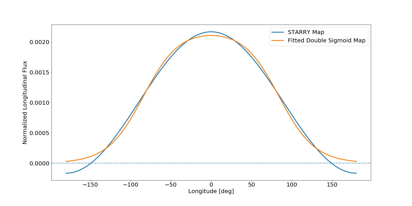
The orange map (“Fitted Double Sigmoid”) was derived by fitting our double sigmoid function above (with scipy.optimize.minimize) to the integrated longitudinal map provided by STARRY (see code snippet below).

from scipy.optimize import minimize
from functools import partial

from starry import kepler, Map

from pylab import *; ion()
import numpy as np
try:
    import exomast_api # pip install git+https://github.com/exowanderer/exoMAST_API
except:
    !pip install git+https://github.com/exowanderer/exoMAST_API
    import exomast_api

def simple_double_sigmoid(params, longitudes): 
    amplitude, scale, shift = params
    
    sigmoid_one = 1/(1+exp(-scale*(longitudes+shift)))
    sigmoid_two = 1/(1+exp(-scale*(longitudes-shift)))
    
    return amplitude*(sigmoid_one - sigmoid_two)

def double_sigmoid(params, longitudes):
    amplitude, scale1, scale2, shift1, shift2 = params

    sigmoid_one = 1/(1+np.exp(-scale1*(longitudes+shift1)))
    sigmoid_two = 1/(1+np.exp(-scale2*(longitudes-shift2)))
    
    return amplitude*(sigmoid_one - sigmoid_two)

def update_starry(system, times, model_params):
    ''' Update planet - system parameters '''
    planet = system.secondaries[0]
    
    edepth = model_params['edepth']
    day2night = model_params['day2night']
    phase_offset = model_params['phase_offset']
    
    planet.lambda0 = model_params['lambda0'] # Mean longitude in degrees at reference time
    planet.r = model_params['Rp_Rs'] # planetary radius in stellar radius
    planet.inc = model_params['inclination'] # orbital inclination 
    planet.a = model_params['a_Rs'] # orbital distance in stellar radius
    planet.prot = model_params['orbital_period'] # synchronous rotation
    planet.porb = model_params['orbital_period'] # synchronous rotation
    planet.tref = model_params['transit_time'] # MJD for transit center time
    
    planet.ecc = model_params['eccentricity'] # eccentricity of orbit
    planet.Omega = model_params['omega'] # argument of the ascending node
    
    max_day2night = np.sqrt(3)/2
    Y_1_0_base = day2night * max_day2night if edepth > 0 else 0
    
    # cos(x + x0) = Y_1_0*cos(x0) - Y_1n1*sin(x0)
    Y_1_0 = Y_1_0_base*cos(phase_offset/180*pi)
    Y_1n1 = -Y_1_0_base*sin(phase_offset/180*pi)
    Y_1p1 = 0.0
    
    planet[1,0] = Y_1_0
    planet[1, -1] = Y_1n1
    planet[1, 1] = Y_1p1
    planet.L = edepth / planet.flux()
    
    system.compute(times)

'''Setup the planet, star, sytem'''
planet_info = exomast_api.exoMAST_API(planet_name='HD 189733 b')

lmax  = 1

phase = np.linspace(0, 1.0, 1000)
times = phase*planet_info.orbital_period + planet_info.transit_time
''' Instantiate Kepler STARRY model; taken from HD 189733b example'''
# Star
star = kepler.Primary()

# Planet
lambda0 = 90.0

planet = kepler.Secondary(lmax=lmax)
planet.lambda0 = lambda0 # Mean longitude in degrees at reference time
planet.r = planet_info.Rp_Rs # planetary radius in stellar radius
planet.L = 0.0 # flux from planet relative to star
planet.inc = planet_info.inclination # orbital inclination 
planet.a = planet_info.a_Rs # orbital distance in stellar radius
planet.prot = planet_info.orbital_period # synchronous rotation
planet.porb = planet_info.orbital_period # synchronous rotation
planet.tref = planet_info.transit_time # MJD for transit center time

planet.ecc = planet_info.eccentricity # eccentricity of orbit
planet.Omega = planet_info.omega # argument of the ascending node

# Instantiate the system
system = kepler.System(star, planet)

# Eclipse depth
fpfs = 1000/1e6

''' Instantiate Kepler STARRY model; taken from HD 189733b example'''
lambda0 = 90.0

model_params = {}
model_params['lambda0'] = lambda0 # Mean longitude in degrees at reference time
model_params['Rp_Rs'] = planet_info.Rp_Rs # planetary radius in stellar radius
model_params['inclination'] = planet_info.inclination # orbital inclination 
model_params['a_Rs'] = planet_info.a_Rs # orbital distance in stellar radius
model_params['orbital_period'] = planet_info.orbital_period # synchronous rotation
model_params['transit_time'] = planet_info.transit_time # MJD for transit center time

model_params['eccentricity'] = planet_info.eccentricity # eccentricity of orbit
model_params['omega'] = planet_info.omega # argument of the ascending node

model_params['edepth'] = fpfs
model_params['day2night'] = 1.0
model_params['phase_offset'] = 0
label='edepth={}ppm; day2night={}; phase_offset={}'.format(model_params['edepth'], 
                                                           model_params['day2night'], 
                                                           model_params['phase_offset'])

update_starry(system, times, model_params)

longitudes = np.linspace(-180,180,1000)
flux_map = np.sum([planet(x=0,y=np.linspace(-1,1,100), theta=theta) for theta in longitudes],axis=1)

flux_map = flux_map / flux_map.sum()

# Fit the Double Sigmoid to the STARRY Longitude Map
def lnprob(params, model, data, data_err):
    
    chisq = ((model(params) - data)/data_err)**2.
    
    return np.sum(chisq)

data_err = 1e-4 * np.ones(longitudes.size)
data = flux_map
partial_model = partial(double_sigmoid, longitudes=longitudes)
init_params = [data.max(), 0.1,0.1,-100, 100]

res = minimize(lnprob, init_params, args=(partial_model,data,data_err))
res = minimize(lnprob, res.x, args=(partial_model,data,data_err))

''' Plot Longitude Map from STARRY '''
fig = figure(figsize=(20,10))
ax = fig.add_subplot(111)

ax.plot(longitudes, flux_map, lw=3, label='STARRY Map')
ax.plot(longitudes, partial_model(res.x), lw=3, label='Fitted Double Sigmoid Map')

ax.axhline(0.0, ls='--')
ax.set_ylabel('Normalized Longitudinal Flux',fontsize=20)
ax.set_xlabel('Longitude [deg]',fontsize=20)

for tick in ax.xaxis.get_major_ticks():
    tick.label.set_fontsize(20)

for tick in ax.yaxis.get_major_ticks():
    tick.label.set_fontsize(20)

plt.legend(loc=0, fontsize=20)

[rodluger]

Related question: how did you derive these equations? I would be interested to try several models in a similar pattern without bothering you; such as the 5 parameter model.

I took the zonal (m = 0) spherical harmonics listed here and got rid of the x and y dependence by substituting z = sqrt(1 - x^2 - y^2), then expressed them in terms of the polar angle cos(theta) = z. So I now have an equation that looks like

I first differentiated it and equated it to zero to find the extrema, and found the relationship between the coefficients that ensured that the minimum occurs at theta = pi and the maximum occurs at theta = 0. Then I found the limits that ensure the function is positive at the minimum.

The hardest equation I had to solve was a quadratic, which leads me to believe that extending this to 3rd order will give me a cubic, which should still be analytic (and 4th order too, theoretically)!

[kevin218]

For today’s motivations, are we suggesting to fit a double-sigmoid function with a set of l=2, 3 spherical harmonics per mcmc step or to derive a relationship between the double-sigmoid and the spherical harmonic coefficients – such as we did for observational parameters vs dipole coefficients in #187?

I mean the latter. There doesn’t seem to be any truly physical reason for the function to be exactly the double sigmoid (right?) so if we find a similarly-behaved l=2 or l=3 spherical harmonic, I can derive the relationship between the coefficients and the observables you care about. I’ll give it a try next week.

The double-sigmoid doesn’t have a singular shape that you can fit once. Its power is in its flexibility to yield sharp gradients (physically motivated by the appearance of clouds) while maintaining a non-negative nightside flux, and expressing the function with a minimal set of free parameters.

I suggest that @exowanderer generates a small subset of representative double-sigmoids that we try to replicate using spherical harmonics. If there is a simple, analytic transformation from one to the other then the additional overhead will be negligible in each mcmc step. Otherwise, we’re likely to lose the speed advantage of moving to spherical harmonics.

Actually, can the integral of a double-sigmoid be computed analytically? Not sure if that’s the primary advantage to using spherical harmonics or if there are other advantages as well.