Time-domain gating: Frequency-domain window required?

This is a branch from the discussion on the mailing list: https://groups.google.com/g/scikit-rf/c/IoH8hNV58sI

Possibly related to issue #734.

The problem is with the roll-off in the edges of the frequency-domain results after gating (at f_min and f_max). A perfectly straight line is provided by PNA transforms. They probably apply a frequency-domain window before the gating.

Discussion: Is this required or advised to do by default?

The theoretical background is covered in an application note by Agilent/Keysight:

• new version; login required
• old version; no login required

Example code based on the data by Roger in the mailing list:

from skrf.media.coaxial import Coaxial
import skrf
import matplotlib.pyplot as plt
import numpy as np

# reflection delays in nanoseconds
t1 = 758.725e-6
t2 = 82.759e-3
t3 = 416.759e-3
t4 = 508.759e-3

# window settings
freq = skrf.Frequency(0.05, 33, 1000, 'GHz')
print(freq.f)
window_type = ('tukey', 0.5)
t_center = t2
t_span = 0.25   # 150 ps

# create network
media = Coaxial(frequency=freq, z0=50)
coax_line_1 = media.line(0.5 * t2, 'ns', z0=50, embed=True)
coax_line_2 = media.line(0.5 * (t3 - t2), 'ns', z0=25, embed=True)
coax_line_3 = media.line(0.5 * t2, 'ns', z0=50, embed=True)
nw_total = coax_line_1 ** coax_line_2 ** coax_line_3

# apply gate
nw_gated = skrf.time_gate(nw_total.s11, window=window_type, center=t_center, span=t_span)

# plotting
fig, ax = plt.subplots(3, 1)

nw_total.s11.plot_s_time(ax=ax[0], label='Original')
nw_gated.s11.plot_s_time(ax=ax[0], label='Gated')
ax[0].set_xlim(-0.5, 1.5)
ax[0].legend(loc='upper right')

nw_total.s11.plot_z_time_step(ax=ax[1], label='Original')
nw_gated.s11.plot_z_time_step(ax=ax[1], label='Gated')
ax[1].set_xlim(-0.5, 1.5)

nw_total.s11.plot_s_mag(ax=ax[2], label='Original')
nw_gated.s11.plot_s_mag(ax=ax[2], label='Gated')
ax[2].set_ylim(0, 1)

plt.tight_layout()
plt.show()

With freq = skrf.Frequency(0.05, 33, 1000, 'GHz'):

With freq = skrf.Frequency(0.05, 330, 1000, 'GHz'):

[RA226]

Keysight reference This document is excellent and I have studied it many times!!! Low-pass and band-pass You are absolutley correct to state that where you can you should use low-pass. I am always thinking in terms of band-pass because I work at such high frequencies. For me the mismatched line is unusual and something I am working on with NPL in the UK and it is in fact their data that you are using with their approval. Convolution or FTT They should be mathematically equivalent but to get the equivalence we have to treat the data correctly. With Roll-off

1. Bandpass FFT with no window causes a roll-off
2. Bandpass Convoltion with Constant or Nearest causes almost identical roll off. This probably depends on exactly where the data stops but it is true in this case.

With no roll-off

1. Bandpass FFT windowed in frequency domain and then remove the window after timegating will remove the roll-off.
2. Bandpass Convolution with Reflect , Mirror, Wrap will also remove the roll-off.

It is easier to visualise why the convolution needs data beyond the last point because as the kernel starts to move past that point the signal will drop-off unless you pad out the data using Reflect or similar. We should always be careful to think about what the final points really mean in this case.

In the FFT case if we do not window the data will have a sharp transition at the edge as it will most likely not be zero. The window forces the data at the edge to go to zero. Then you need to remove it when you transform back.

Windowing in Frequency domain If you window in the frequency domain using Network.windowed before Fourier transforming to the time domain you have to divide the network by the window when you transform back to the frequency domain. So if you used the Network.windowed method with all the defaults you would have to divide by the equivalent window as follows:

Window_full = signal.kaiser(NPoints, beta=6)
S = 0.5 * S_trans_windowed / Window_full
# Needs the factor of 2 to scale the amplitude correctly

I have tested this in the past and it works fine.

How to proceed My view would be:

1. Adding a low-pass option is a good idea
2. Use FFT and have it windowed by default. The inverse window could be provided as another method of Network.
3. Be able as an option to switch off windowing
4. There maybe some cases where convolution provides advantage. In my tests with 15mm silica in freespace (75-110 GHz) the FFT method gave some ringing which is worse at the edge of the band but this was not seen in convolution as shown below.

[Vinc0110]

Ok, things have been really confusing, but I think I sorted it out. Various different topics got mixed, all described very well in the application note by Agilent linked above:

• frequency-domain truncation and windowing: the measured frequency span would ideally be infinite, but it is obviously limited in real-world applications. This causes widening of peaks, sometimes even large ripples in the time-domain responses after the IDFT/IFFT. Applying a (non-rectangular) window function to the frequency-domain data helps mitigating this effect. scikit-rf already has a feature for this: Network.windowed(). This is fine for (visual) analysis of the time-domain response, but results in total garbage if that response gets transformed back into frequency domain (e.g. after time gating).
• time-domain low-pass mode: taking the IDFT/IFFT on positive and negative frequency samples with the negative part being a complex-conjugate copy of the positive part (hermitian response), including the dc component. This results in a real-valued time-domain signal. irfft() and rfft() from numpy.fft do exactly this.
• time-domain band-pass mode: taking the IDFT/IFFT only on the positive frequency samples, generally without the dc component. This results in a complex-valued time-domain signal. The regular ifft() and fft() from numpy.fft do exactly this.

The current implementation of time_gate() performs time-domain band-pass mode. What we see is actually in line with the statements in Agilent’s application note linked above:

The IFT is applied from minus one-half of the frequency span to plus one-half of the span. This windows both sides of the data which increases the impulse width and reduces the effective bandwidth. The fact that the response is centered around the VNA center frequency has the effect of multiplying the normal time domain response by a “modulation” function producing a sinusoidal wave on top of the normal response. This is apparent in bandpass mode, real or imaginary formats, but is eliminated in the log mag or lin mag format. In contrast, the center of the windowing function in the low- pass mode is the DC term, or the first point of the data set. Compared to the low-pass mode, for the same frequency span and number of points, bandpass mode has twice the impulse width, which may obscure closely spaced responses.

Sorry for all the plots, but it’s really interesting to compare different setups. As you will see, the overall frequency span of the measurement and the (relative?) span of the window has a big impact. The type of window is not too important and only influences the ripple.

---

Setup 1: freq = skrf.Frequency(0, 330, 1001, 'GHz')

Plot 1.1: comparing the time-domain responses using low-pass mode, band-pass mode, and the current skrf implementation (normal and windowed):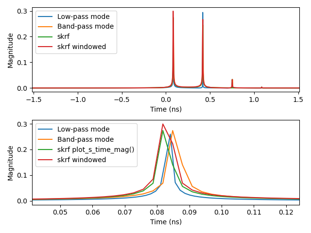

Plot 1.2: Gating the first reflection using low-pass and band-pass transforms with a Hann window: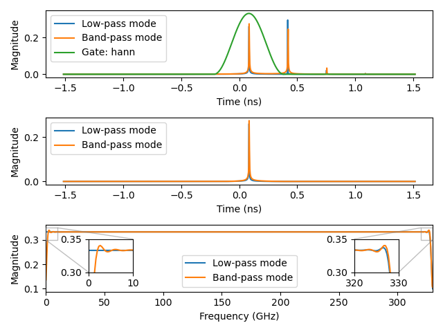

Plot 1.3: Gating the first reflection using low-pass and band-pass transforms with a Kaiser window (beta=10):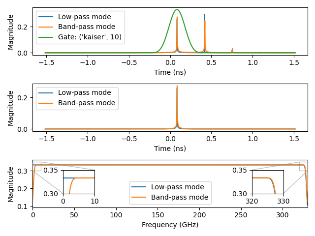

Plot 1.4: Gating the first reflection using low-pass and band-pass transforms with a Tukey window (alpha=0.6):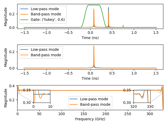

---

Setup 2: freq = skrf.Frequency(0, 33, 1001, 'GHz')

Plot 2.1: comparing the time-domain responses using low-pass mode, band-pass mode, and the current skrf implementation (normal and windowed):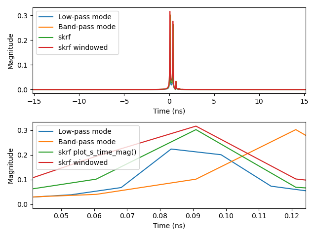

Plot 2.2: Gating the first reflection using low-pass and band-pass transforms with a Hann window: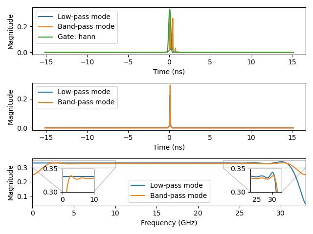

Plot 2.3: Gating the first reflection using low-pass and band-pass transforms with a Kaiser window (beta=10):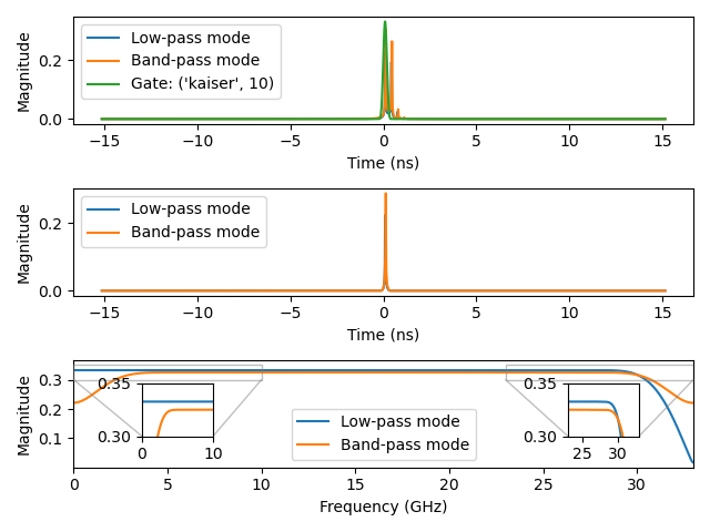

Plot 2.4: Gating the first reflection using low-pass and band-pass transforms with a Tukey window (alpha=0.6):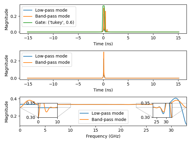

---

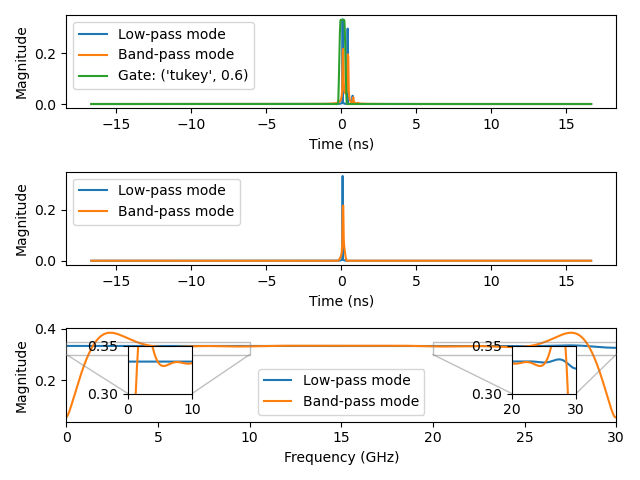
Setup 3: freq = skrf.Frequency(0, 30, 1001, 'GHz')

Plot 3.1: comparing the time-domain responses using low-pass mode, band-pass mode, and the current skrf implementation (normal and windowed):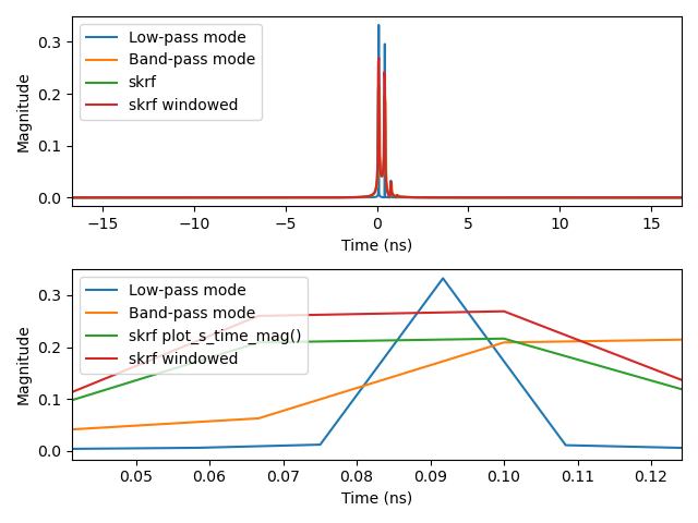

Plot 3.2: Gating the first reflection using low-pass and band-pass transforms with a Hann window: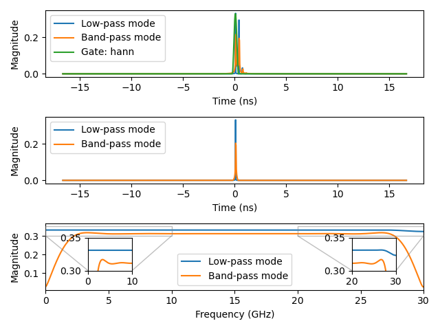

Plot 3.3: Gating the first reflection using low-pass and band-pass transforms with a Kaiser window (beta=10):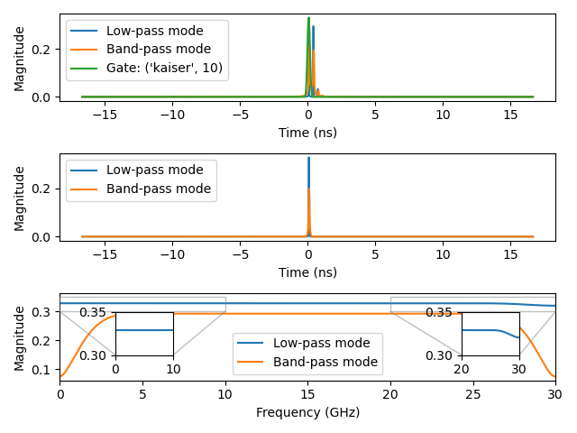

Plot 3.4: Gating the first reflection using low-pass and band-pass transforms with a Tukey window (alpha=0.6):