Easily plot and compare multiple marginal posteriors

I wanted a way to efficiently compare multiple marginal posteriors in PyMC3/ArviZ like in Figure 9.10 from Kruschke’s book:

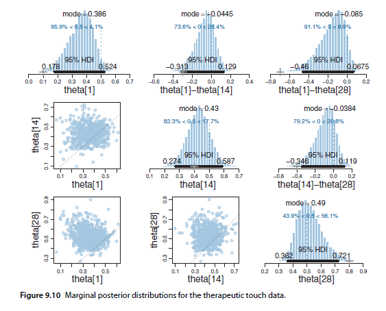
This is especially the case when using vectorized parameters in a model, and I’d like to compare many/all of them. If I have two, creating a pm.Deterministic difference isn’t bad.

I searched PyMC3/ArviZ documentation and examples, and didn’t seem to find anything that fit this need. Forest plots give similar answers, but comparing HPDs of two parameters is not the same as looking at the HPD of their difference.

I created a function to plot the difference in marginal posteriors.

from matplotlib import pyplot as plt
import numpy as np
import pymc3 as pm
import arviz as az


def compare_posterior(
    trace,
    var_name,
    triangle="lower",
    identity=True,
    figsize=None,
    textsize=None,
    credible_interval=0.94,
    round_to=3,
    point_estimate="mean",
    rope=None,
    ref_val=None,
    kind='kde',
    bw=4.5,
    bins=None
):
    triangle_options = ("lower", "upper", "both")
    assert (
        triangle in triangle_options
    ), f"triangle argument must be 'lower', 'upper' or 'both'."
    
    num_param = trace[var_name].shape[1]
    if figsize is None:
        figsize=(num_param * 2.5, num_param * 2.5)
        
    fig, axes = plt.subplots(num_param, num_param, figsize=figsize)
    for i in range(num_param):
        for j in range(num_param):
            ax = axes[i, j]
            if triangle is "lower" and i < j:
                ax.axis("off")
                continue
            elif triangle is "upper" and i > j:
                ax.axis("off")
                continue

            if i is not j:
                az.plot_posterior(
                    trace[var_name][:, i] - trace[var_name][:, j],
                    ref_val=ref_val,
                    ax=ax,
                    textsize=textsize,
                    credible_interval=credible_interval,
                    round_to=round_to,
                    point_estimate=point_estimate,
                    rope=rope,
                    kind=kind,
                    bw=bw,
                    bins=bins,
                )
                ax.set_xlabel(f"{var_name}_{i} - {var_name}_{j}")
            else:
                if identity:
                    az.plot_posterior(
                        trace[var_name][:, i],
                        ax=ax,
                        textsize=textsize,
                        credible_interval=credible_interval,
                        round_to=round_to,
                        point_estimate=point_estimate,
                        kind=kind,
                        bw=bw,
                        bins=bins,
                    )
                    ax.set_xlabel(f"{var_name}_{i}")
                else:
                    ax.axis("off")
    plt.tight_layout()
    return axes

# Generate data
N = 1000
W = np.array([0.35, 0.4, 0.25])
MU = np.array([1.8, 2., 2.2])
SIGMA = np.array([0.5, 0.5, 1.])
component = np.random.choice(MU.size, size=N, p=W)
x = np.random.normal(MU[component], SIGMA[component], size=N)

# Build and run model
with pm.Model() as model:
    # define priors
    mu = pm.Uniform('mu', lower=0, upper=10, shape = MU.size)
    sigma = pm.Uniform('sigma', lower=0.001, upper=10, shape=MU.size)
    # likelihood
    likelihood = pm.Normal('likelihood', mu=mu[component], sd=sigma[component], observed=x)
    trace = pm.sample(2000, tune=2000, cores=2, chains=3)

# Plot
compare_posterior(
    trace,
    var_name="mu",
    triangle="lower",
    ref_val=0,
    credible_interval=0.95,
)
plt.show()

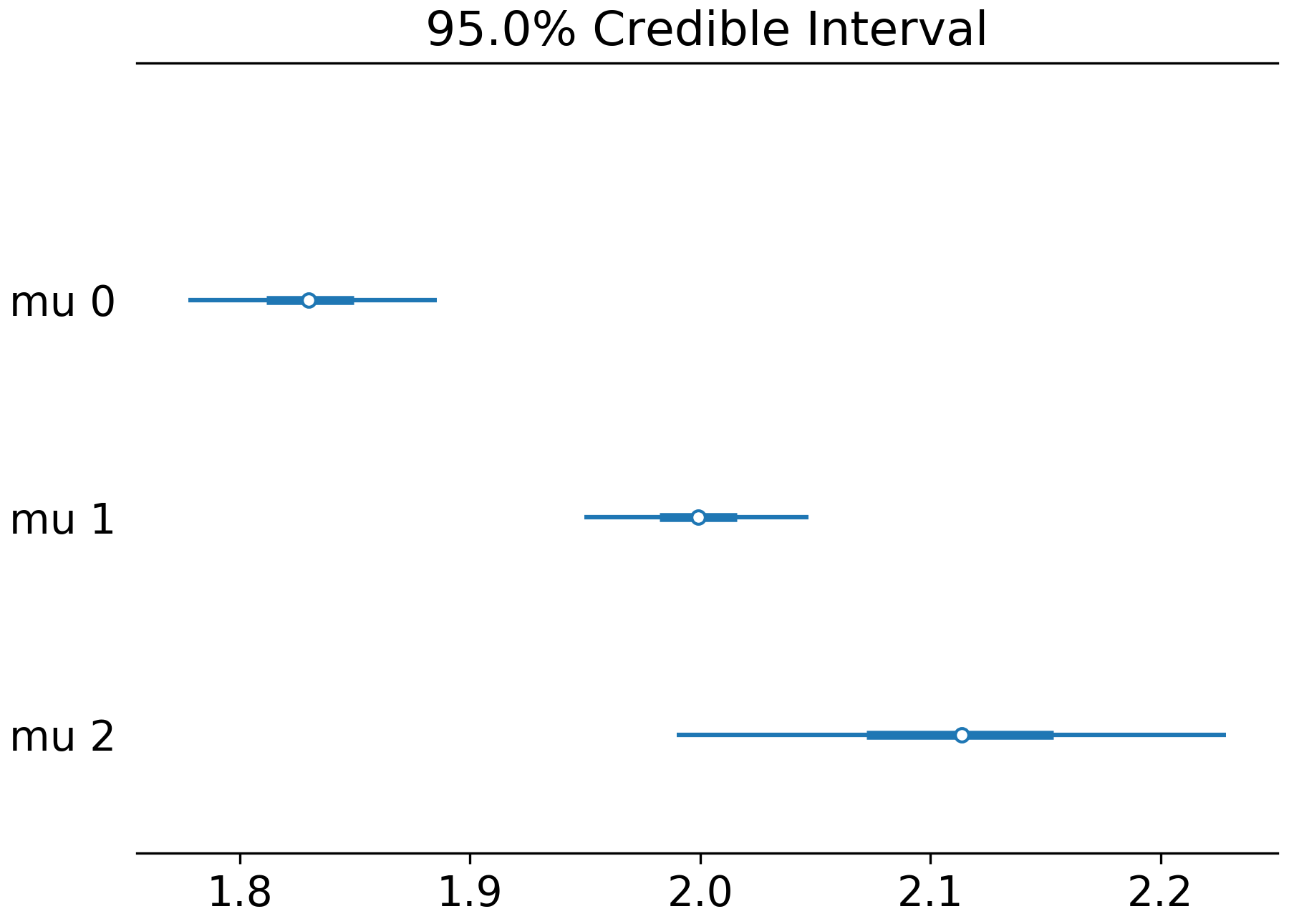
Here’s the combined forest plot for the same trace:

I didn’t care about recreating the scatter plots, but the function could be modified to faithfully recreate the original figure:

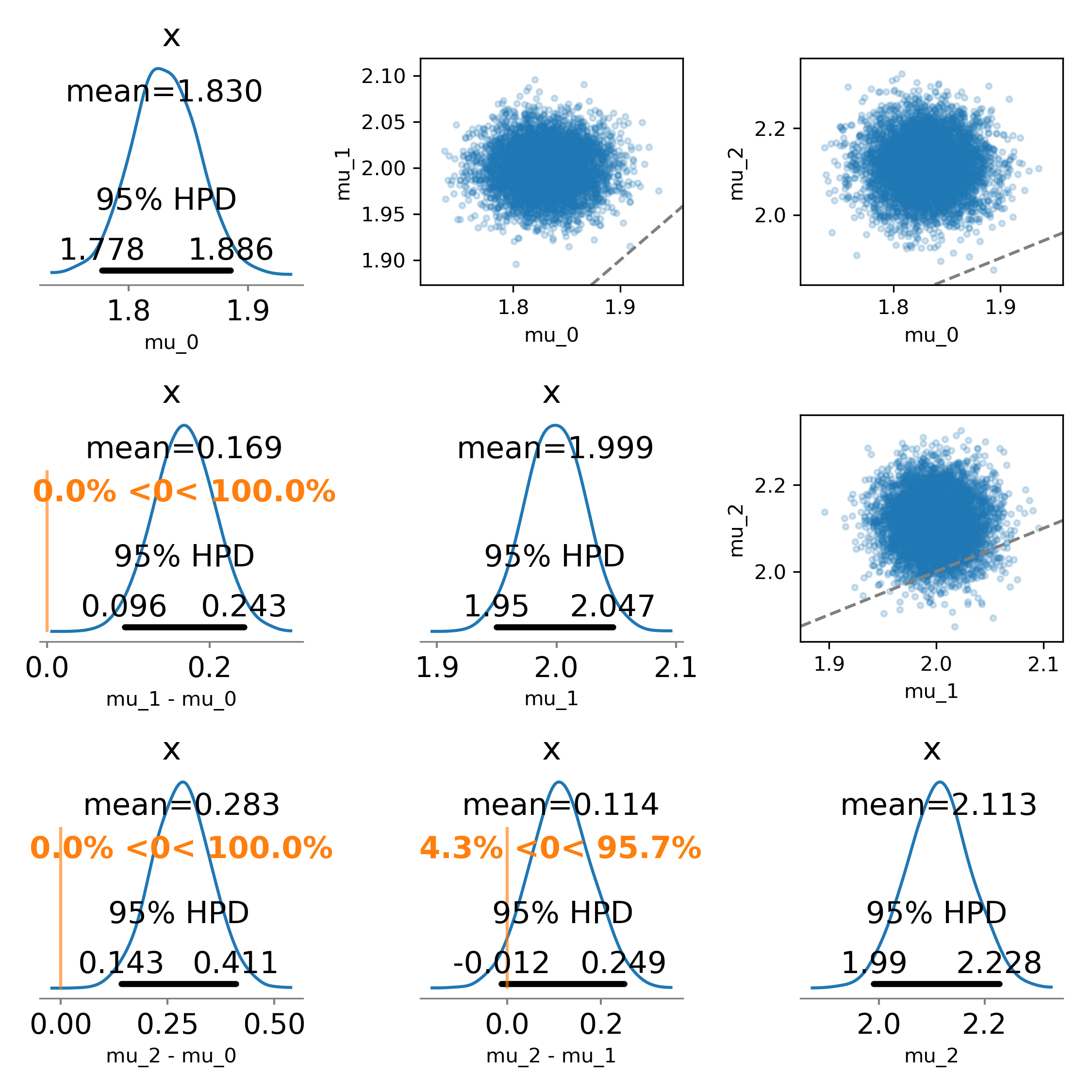
The results (and interpretations) may be different from what you’d get from a forest plot, depending on the data and parameters.

My function assumes that only one parameter would be compared at a time, and assumes that the parameter vector is a reasonable length. It’s a little hackish, and assumes a PyMC3 trace for data.

Is this something worth adding to arviZ? Is there any reason that these types of plots are invalid or shouldn’t be encouraged? If there’s interest, I’d be willing to build this into a PR to add to arviZ (and PyMC3 plotting).

[hectormz]

@aloctavodia I’ll work on a PR that follows the current format as existing plots. Thanks! I’ll check in if I have questions.

[aloctavodia]

Hi @HectorM14 thanks for this contribution, the plot looks really nice. It will be really great if you send a PR with this new plot. Please use our existing plots as a reference, maybe pair_plot is a good place to check.