Eclipse depth vs Phase Curve Ampitude

Motivation I am trying to use the system.lightcurve in starry with my emcee implementation to fit a starry phase curve model to my Spitzer photometry.

Background When I ran a MCMC analysis on existing Spitzer+Phase Curve code (skywalker), I found that the eclipse depth with STARRY was roughly twice the eclipse depth measured using only a cosine function for the phase curve; i.e:

ang_freq = 2*pi/period
phase_curve = half*cosAmp*np.cos(ang_freq * (times - (t_secondary - cosPhase)))

[Sidenote: The half in my formula is critical because the “amplitude” I want to measure is the top - bottom of the flux at the eclipse location. The result is that the measurement of “cosAmp” is the top - bottom of the phase curve; and the cosPhase provides the adjustment to “at the eclipse location”]

Issue I want to use STARRY to interpret the eclipse depth, phase curve amplitude, phase curve offset, night flux, and orbital parameters (e.g. eccentricity, a/Rs, etc) from the MCMC fit of the phase curve.

The figure below shows three different phase curves:

1. (blue) with no eclipse and no phase curve amplitude
2. (orange) with an eclipse (FpFs=1000ppm) and no phase curve amplitude
3. (green) with an eclipse (FpFs=1000ppm) and phase curve amplitude set to 1.0 (Y_1_0 = 1.0).

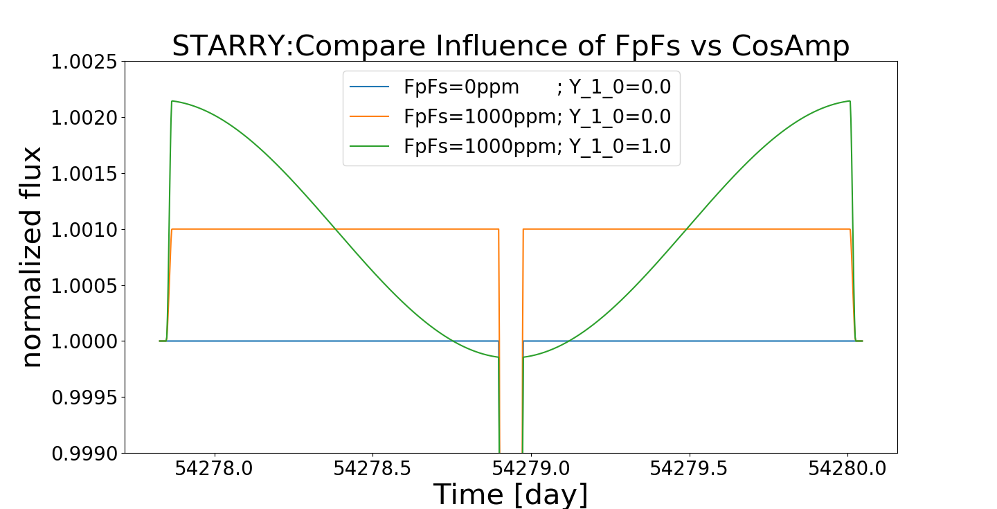
In this figure, an observer would say that that the

1. “eclipse depth of the blue curve is 0.0”
2. “eclipse depth of the orange curve is 1000ppm”
3. “eclipse depth of the green curve is 2200ppm”

Unfortunately, the input that I used for the eclipse depth to both the orange & green curves was identical (FpFs = 1000ppm).

I would expect – because the phase curve offset is zero – that the difference between the top and bottom of the green curve should be identical to the difference between the top and bottom of the orange curve.

The “eclipse depth” is the loss of flux during eclipse; but (I think) the MCMC enters the eclipse depth as a free parameter (planet.L below) and the phase curve amplitude (planet[1,0] below) as an independent free parameter.

In the end, the MCMC shows that planet[1,0] and planet.L are strongly correlated (Pearson > 0.9), which is intuitive; but for zero phase curve offset and no night flux, the eclipse depth should equal the day-to-night variation; here the day-to-night side variation is greater than twice the entered eclipse depth.

To an observer, if I provide a model with the fpfs (see below) and cosAmp (half day-to-night variation) – at no phase curve offset and no night flux – I would expect the orange curve to reach maximum at the top of the eclipse and reach minimum at the top of the transit. The green starry curve has a maximum >2x larger the than maximum for the orange curve; and a minimum below the bottom of the orange/green eclipse.

I think that the issue is, as an observer, I want to interpret planet[1,0] as the day-to-night variation (~phase curve amplitude) and planet.L as the eclipse depth (~Fp/Fs).

[tl;dr]: Could you guide me on how to infer the physical parameters (eclipse depth & phase curve amplitude) from the STARRY light curve results?

[Related side note: The flux at the top of the transit should never be less than the flux at the bottom of the eclipse; see green curve < blue curve at transit.]

---

Here is a code snippet to reproduce this figure:

from starry import kepler

from pylab import *; ion()
import numpy as np
import exomast_api # pip install git+https://github.com/exowanderer/exoMAST_API
planet_info = exomast_api.exoMAST_API(planet_name='HD 189733 b')

lmax  = 1

''' Instantiate Kepler STARRY model; taken from HD 189733b example'''
# Star
star = kepler.Primary()

# Planet
lambda0 = 90.0

planet = kepler.Secondary(lmax=lmax)
planet.lambda0 = lambda0 # Mean longitude in degrees at reference time
planet.r = planet_info.Rp_Rs # planetary radius in stellar radius
planet.L = 0.0 # flux from planet relative to star
planet.inc = planet_info.inclination # orbital inclination 
planet.a = planet_info.a_Rs # orbital distance in stellar radius
planet.prot = planet_info.orbital_period # synchronous rotation
planet.porb = planet_info.orbital_period # synchronous rotation
planet.tref = planet_info.transit_time # MJD for transit center time

planet.ecc = planet_info.eccentricity # eccentricity of orbit
planet.Omega = planet_info.omega # argument of the ascending node

planet[1,0] = 0.0 # Y_1_0

# System
system = kepler.System(star, planet)
# Instantiate the system
system = kepler.System(star, planet)

# Specific plottings
fpfs = 1000/1e6
Y_1_0 = 1.0

phase = np.linspace(-0.5, 0.5, 1000)
times = phase*planet_info.orbital_period + planet_info.transit_time

fig = gcf()
ax = fig.add_subplot(111)
system.compute(times)
ax.plot(times,system.lightcurve)

planet.L = fpfs
system.compute(times)
ax.plot(times,system.lightcurve)

planet[1,0] = Y_1_0
system.compute(times)
ax.plot(times,system.lightcurve)
ax.set_ylim(1-fpfs,1 + 2.5*fpfs)

ax.set_xlabel('Time [day]', fontsize=30)
ax.set_ylabel('normalized flux', fontsize=30)

ax.set_title('STARRY:Compare Influence of FpFs vs CosAmp', fontsize=30)

ax.legend(('FpFs=0ppm      ; Y_1_0=0.0', 
                     'FpFs=1000ppm; Y_1_0=0.0', 
                     'FpFs=1000ppm; Y_1_0=1.0'),loc=0, fontsize=20)

for tick in ax.xaxis.get_major_ticks():
    tick.label.set_fontsize(20)
for tick in ax.yaxis.get_major_ticks():
    tick.label.set_fontsize(20)

[rodluger]

@exowanderer Thanks for the awesome issue description. I’ll play around with things a bit this morning, and we can chat throughout the day, but right off the bat I think the issue is with your interpretation of the Y_{1,0} harmonic. That harmonic is symmetric about the plane of the sky, so whatever flux you are adding to the dayside, you are also subtracting it from the night side. So by setting Y_{1,0} = 1.0, you are effectively giving the planet negative flux on the night side, which explains why the phase curve dips below 1 near transit.

Also, all Primary and Secondary map instances have the constant Y_{0,0} term fixed at unity (which is something I’m considering changing & we can chat about), so by also setting the Y_{1,0} coefficient to unity, you are effectively doubling the brightness of the dayside. That’s why the eclipse depth of your green curve is about twice that of the orange curve. If you want them to be the same, you should probably adjust the luminosity of the body. So you could probably get what you want – matching eclipse depths – by decreasing the overall luminosity of the planet when plotting the green curve. We can probably sit down and figure out the math behind all this so you don’t have to eyeball it.

I think that the issue is, as an observer, I want to interpret planet[1,0] as the day-to-night variation (~phase curve amplitude) and planet.L as the eclipse depth (~Fp/Fs).

Ah, yes, that’s exactly the issue! planet.L is the 4-pi steradian integrated intensity (i.e., the actual luminosity), which is different from the eclipse depth. And planet[1,0] is the strength of the dipole term, which is proportional to the phase curve amplitude. Let’s sit down today and chat more about our definitions and try to find a bridge between our conventions.

[rodluger]

@exowanderer I’ll poke around your code a bit, but as per our conversation this morning, this is how you add a 30 degree longitudinal offset to the dipole map:

map = starry.Map()
map[1, 0] = 0.5
map.axis = [0, 1, 0]
map.rotate(-30)
map.show()